Chapter 5 - Excel Basics

5.7 Building a Function

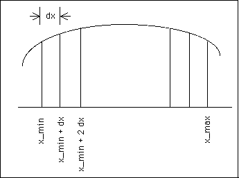
Excel can only deal with numbers and table of numbers. Therefore, to build and plot a function requires to first build a table of values for the function, and then to plot the table. Conceptually, this is equivalent to introducing a numerical grid, i.e., a set of values of the independent variable at which the function is evaluated. This is illustrated in the following cartoon for an equally spaced grid:

The numerical grid is defined by the domain (range) of the independent variable, x={x_min,x_max}, and by the number of grid points, N_grid, from which one deduces the grid spacing, dx. This is illustrated above. In this case

dx = ( x_max - x_min ) / ( N_grid - 1 )

Equivalently, one could specify x_min, dx, and N_grid, from which x_max can be deduced, or any consistent combination of these variables. For instance, a person observing the value of a stock twice a day, dt=dx=0.5 day, for for 30 days could define t_min=x_min=0 and t_max=x_max=30 days and deduce that N_grid=61.

In the following, we will use Excel to build the function f(x) = a x ^b. We will assume a and b to be initially given ( a = 1.2 and b = 1.7 ); these values are what defines the function. The range in x will be initially given as x={0,2}. We want to design an Excel spreadsheet in which the function definition and x range can be adjusted arbitrarily.

The steps are

5.7.1 Build the numerical grid

5.7.2 Tabulate and Plot the Function

5.7.3 Set the appearance of the final spreadsheet for printing

This example illustrates the procedure to build and plot any function using Excel. The basis for doing so is the evaluation of the function on a numerical grid.

You may want to download the spreadsheet we just built: for the Mac or for the PC platform. This will allow you to experiment somewhat more with the subtleties of Excel in building such a spreadsheet.

Adding a function ( or many functions ) to our spreadsheet should now be easy to do. For instance, plotting simultaneously f(x)=x² ( a = 1.0 and b = 2.0 ) and sin(x) is illustrated in Section 5.7.4.

Any questions or suggestions should be directed to Michel Vallières at vallieres@physics.drexel.edu