
Data sets are not always best fitted by straight lines. In particular, there are two types of functional forms that can easily be fitted by a straightforward extension of the linear regression using Excel: the power law and the exponential law.
![]() power law
power law
![]() exponential
law
exponential
law
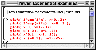
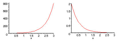
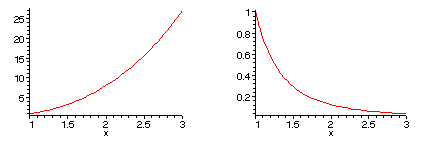
These provide a great variety of "shapes" with which to fit a data set. For example, the following Maple worksheet illustrates some of these forms:

This extend our choices to the linear law, the power law or the exponential law to fit any given data set. The choice is solely dictated by which data set will fit the data better.
The power law is
![]()
where a and b are two parameters to adjust so as to produce the best fit to a given data set.
Finding a and b can be related to the linear regression via a simple trick. Take the natural logarithm of both sides of the equation:
![]()
This leads to the "log-log" plot, whereby ln(y) is plotted versus ln(x). The power law then produces a straight line dependence. Namely, ln(y) versus ln(x) is analogous to
![]()
where "y" is taken as "ln(y)" and "x" is taken as "ln(x)". The parameters a and b are then found to be related to the slope and intercept of the line via
![]()
The following Excel spreadsheet illustrates this "straightening out" effect via the function f(x) = x 3 . The function f(x) is first plotted versus x; ln( f(x) ) versus ln(x) is then plotted. We see the straight line as expected.

Given a noisy data set, a power law fit is then archived via the following steps:
The exponential law is given by:
![]()
Taking the natural logarithm of both sides yields
![]()
This is analogous to the straight line equation
![]()
provided that "y" is taken to be ln(y) and that "x" remains "x". This yields to notion of a "semi-log" plot, whereby ln(y) is plotted versus "x". The parameters a and b are then found to be related to the slope and intercept of the line via
![]()
The fit is obtained via the following steps:
![]() Any questions or suggestions should be directed to
Any questions or suggestions should be directed to
Michel Vallières at vallieres@einstein.drexel.edu