

Mathematical modeling is often associated with initial value problems in which the initial value of a or many variables are specified and the time evolution of these variables sought. The problem is then defined by specifying the rates of change of the variables with time. If these rates are only functions of the independent variable, the time, then the solution of the equations are simple integrals. For instance, if f(t) is the function we want to find given that it satisfies the equation
![]()
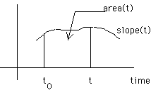
The solution for the function f(t) is then the "area" under the curve, when calculated from tinitial to t, i.e.,

Geometrically,

This area can be found via numerical methods, i.e., the trapezoidal rule, or analytically via the Maple command "int" if the RHS function is known analytically (and not so complicated!). The syntax for calculating an analytical solution is
f := unapply( int( slope(t), t=t_initial..T ), T );
The situation is very different if the rates of change are themselves functions of the unknown functions, i.e.,
![]()
In this cases, the simple idea of calculating the "area" under a "curve" is not possible since the "curve" can not be drawn since it itself depends on the unknown function f(t). The solution of such equations is notoriously more complicated.
These type of equations are called differential equations. They are at the heart of most mathematical modeling, whether it deals with physics, or chemistry, engineering, biology, epidemics, finance, ...
Any questions or suggestions should be directed to
![]() Chapter 8
Chapter 8
![]() Section 8.2
Section 8.2
![]() TOC
TOC
![]()
Michel Valličres at vallieres@physics.drexel.edu