Chapter 3 - Solving Algebraic Equations

3.2 Graphical Interpretation

Solving one or more algebraic equations can be interpreted graphically as finding the intersections of curves. For instance, solving

x ^x = 100

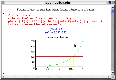
is interpreted as finding the intersection of the graph of the function f(x) = x ^x with the graph of the constant function g(x) = 100. The worksheet below contains a graph of these two functions. Let your eyes follow the two curves, and find x at which the two curves intersect, x_soln. The values of the functions at that point are evidently f(x_soln) = g(x_soln). Note that in general there could be many intersections.

\

In the worksheet above, a vertical line in inserted on the graph using the solution x_soln to confirm that the solution found by Maple really corresponds to the x-coordinate of intersection point. To plot this line, the "plot" command is used with the point list form, i.e., [ [x₁,y₁], [x₂,y₂], ... ] where the pair of coordinates [x_k,y_k] points to the k^th point in the x-y plane.

Systems of Equations

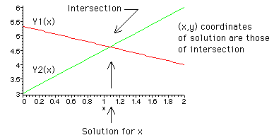
The same applies to solutions of systems of equations. Each equation specifies a relation between variables in the multi-dimension space of the variables, i.e., graphs, and the solutions corresponds to the intersection of the curves.

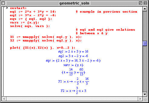
The following set of 2 equations containing 2 unknowns (x,y) specify two relations between x and y, labeled Y1(x) and Y2(x) in the worksheet. The latter are obtained by solving for y as a function of x for each of the two equations. "unapply" is used to make functions out of Y1(x) and Y2(x) since these functions are Maple generated. Y1(x) and Y2(x) are straight lines since the original equations were linear in x and y. The plot of Y1(x) and Y2(x) show these straight lines to intercept. The solution of the system of equations corresponds to finding the intersection between the two curves.

Any questions or suggestions should be directed to Michel Vallières at vallieres@physics.drexel.edu