Deep Learning From First Principles

Goal and Purpose

Linear regression is the simplest and arguably most well-known form of machine learning.

Linear regression models, as in statistics, are concerned with minimizing error and making the most accurate predictions possible. A neural network can accomplish this by iteratively updating its internal parameters (weights) via a gradient descent algorithm. The Youtube educator 3B1B has a great visualization of gradient descent in the context of machine learning models.

In this notebook, I will develop a simple single-layer model to “learn” how to predict the outcome of a linear function of the form y=mx+b. This excersize may seem trivial or unecessary (“I can produce a list of solutions for a linear function and plot it with a few lines of code, why do I need a neural network to try and learn how to do the same thing?”) but this will act as a backbone to build more complex neural networks for much much more complicated functions.

We will start with the simplest possible neural network, one input neuron and one output neuron with which we will learn how to create linear functions. Then, we will expand upon this simple model by allowing for multidimensional inputs (andd thereby allowing for multidimensional outputs as well). Finally, we will complete our foray into Deep Learning by adding “hidden layers” to our neural network. The result will be a modular Deep Learning model that can be easily applied to a diverse set of problems.

The Simplest Neural Network

A neural network can be thought of as a function: input, transformation, and output. Therefore, in its most simple representation, a neural network can take a single input, produce an output, and by comparing that output with the known result, can update its internals to better approach the correct output value.

Here, x is some input number, the input is transformed via our neural network function which has parameters W and b (weight and bias). These parameters are subject to change based on how erroneous the network’s output $\hat{y}$ is compared to the actual value we’d expect from input x.

The simple neural network has the following steps:

1. Initialize training input x_train and output y_train. The output here is the expected correct answer.
2. Initialize network parameters W and b . Here the weight array must correspond to the number of inputs. Since we only feed in one input at a time for now, the weights and bias arrays will have shape (1,1). The weight is initialized to a small random number.
3. Define our cost function. The “cost” can be thought of as the error between the expected output and our network’s output. “Cost” and “Loss” are similar, though I believe the Loss function is the averaged error when considering a multitude of simultaneous inputs. We’ll showcase this later, for now, each error calculation is refered to as the cost.
4. Calculate the components of the gradient of the cost function. In this case: $\frac{\delta W}{\delta C}$ and $\frac{\delta b}{\delta C}$
5. Update the network parameters by reducing by a scaled amount of the gradient components. This is gradient descent.
6. Repeat this process any number of times, called epochs. Return the parameters W and b.
7. Use the model’s updated parameters on test data to determine how accurate the trained model is.

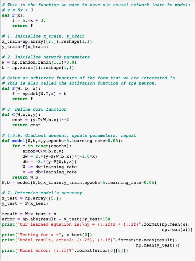
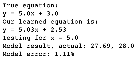
Wonderful! By just feeding our neural network the same number over and over again (5 times in total), we were able to train the network to respond to any other number to within ~1% error.

In Neural Network models, we refer to the weights and biases of the model as the model’s parameters. These are elements that change throughout the model’s learning process but that we do not necessarily have direct control over. Number of learning iterations (epochs) and the learning rate (which scales by how much parameters W and b are changed) are examples of hyperparameters. We typically DO have direct control over hyperparameters. Below, we can see the effect of a decreased learning rate and increasing epoch number.

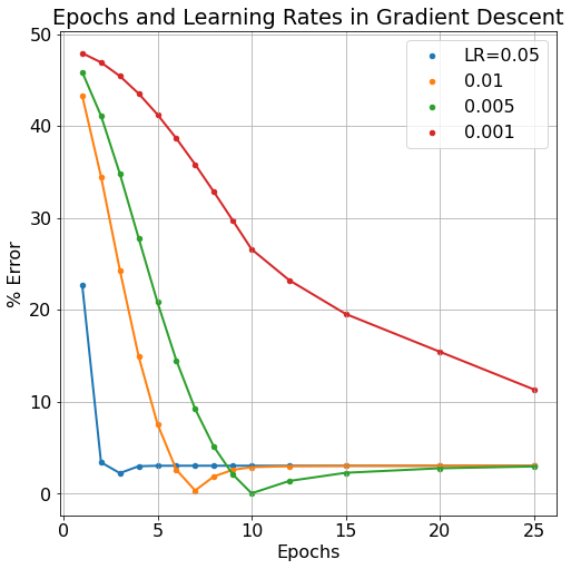
Typically, we’d expect more epoch iterations to lend to less model error since it gives more iterations to improve the model parameters. But this can also have a detrimental effect as the model becomes “over-trained”. The learning rate can also be over-tuned, if the learning rate is too large, the model will bounce around it’s cost/loss minimum without ever “descending the gradient”. If the learning rate is too small, the model will learn very accurately but very slowly, requiring many more epoch iterations to get equivalent results to larger learning rates. As can be seen in the figure below, more epochs can sometimes cause a model’s error to rise while smaller learning rates take more epochs to improve.

An Expanding Parameter-Space

An easy way to expand the complexity of our simple neural network (and take another step towards a much more complex deep learning network) is to allow for multi-dimensional inputs. In this case, we can have our model train on 5 values at a time rather than just a single value as before. This can be thought of as training a model to recognize a collection of pixels rather than just a single one, certainly an important progression.

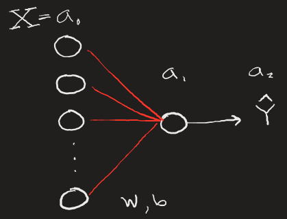
To make compounding improvements, we want to be able to pass multiple inputs into our neural net without having to loop over the input values. We can do this fairly simply by:

1. Establishing our training set as some (1,n) shaped array, with n=5 here. (We can change this later when we add more training examples, think m images with n pixels).
2. Ensuring our parameters W and b reflect the correct dimensions of the incoming multi-dimensional input. Here, those dimensions must be (1,n) since there must be n parameters going to 1 output node.
3. Averaging our gradient calculations for dw and db since our gradient calculation with produce (n,n) matrices for both. We can collapse them to (1,n) arrays and divide by the number of parameters n.

These changes can be seen in the following code snippet (compare to our “simplest” neural network from before). The network output is a little more complicated, as now we now can see the error for each of the n parameters needed for our model to train. In a way, we are training n linear equations at the same time.

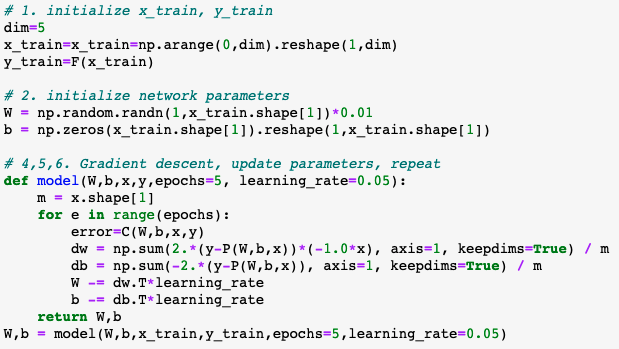
The behavior of our models parameters under the shift of the learning rate and epoch number hyperparameters is expectedly improved compared to our “simplest” moedl. Although it’s difficult to quantify exactly how this expanded model has improved itself more efficiently, we can certainly see that the model trains to an equally “good” level of low error in less epochs than our previous simple model and that even at the lowest learning rate level our new model can learn more efficiently.

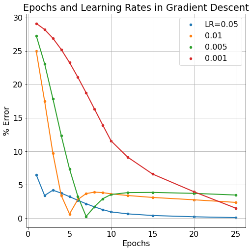
Though we still see similar macro-trends in our new and improved model: it’s still possible to over-train the model, and too low of a learning rate can increase the learning iterations needed, thereby requiring undue computational requirements.

Next, we’ll expand on our neural network once more, this time adding so-called “hidden layers” to the network which will further improve the model’s learning capabilities.