Step into the Deep(Learning)
What Makes Learning “Deep”?
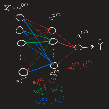
It’s important to recognize the profound difference between the models we have built up until now and this current iteration. Previously, we our most advanced model relied on any number of hidden layers consisting of a single node. We found that such a model can still “learn” simple linear functions, but we would not expect a series of linear 1D transformations to be able to model any complex funcitons such as those involved in image recognition.
Expanding each layer into any number of neurons allows for multi-dimensional linear transformations that aid in the extraction of complex patterns within data, decomposing a set of information into otherwise invisible correlations. Once a neural network has the structure necessary to greatly decompose a data set, it becomes much easier for the network to learn from the data, both in time spent learning and the network’s ability to accurately respond to new data once the learning is complete.

Coding in the Deep
The code behind coupling high-dimensional neural network layers is surprisingly simple. At its core, transforming activations to a new layer is a linear matrix transformation, one that can be performed quickly and in a single line of code using numpy. The N-dimensional layer can also be built easily with native numpy routines. The most difficult part of this process is the bookkeeping: keeping track of each neuron’s weight, bias, and activation as well as the corresponding gradient descent information for the backpropogation step. As a neural network expands, the size of the book to be kept becomes enourmous. Luckily, it’s straightforward to build a dictionary to maintain the activation and gradient descent data and ensure that it loops over and includes all data reguardless of any number of layers or number of neurons within individual layers.
def L_layer_model(X, Y, layer_dims, learning_rate=0.05, num_iterations=10, print_cost=False):
    np.random.seed(2)
    costs = []
    # 0. Initialize parameters
    parameters = init_parameters(layer_dims)
    m = Y.shape[1] # used for cost calculation

    # 0a. Loop gradient descent
    for i in range(0, num_iterations):
        # 1. Forward Propogation.
        # Get activation of layer L and the cache of intermediate parameters and neuron values.
        caches = []
        A = X
        L = len(parameters) // 2
        for l in range(1,L):
            # Starting from 1 since layer 0 is the input layer.
            A_prev = A
            A, cache = linear_activation_forward(A_prev, parameters['W'+str(l)], parameters['b'+str(l)], 'none') #usually relu
            caches.append(cache)
        # Calling forward activation on last layer separately so we can use sigmoid activation function.
        AL, cache = linear_activation_forward(A, parameters['W'+str(L)], parameters['b'+str(L)], 'none')
        caches.append(cache)

        # 2. Compute Cost
        cost = compute_cost(m, AL, Y)
        cost = np.squeeze(cost) # squeezes out value from weird numpy array format (e.g turns [[17]] to 17).
        costs.append(cost)
        if (print_cost):
            print("Cost is {:.2f} on iteration {}".format(cost, i))

        # 3. Backward Propogation: get gradients
        grads = {}

        Y = Y.reshape(AL.shape) # Y and AL are now same shape

        dAL = -2.0*(Y-AL) # Derivative of Loss function with respect to final layer activation AL

        # Lth layer (Sigmoid --> Linear) gradients
        current_cache = caches[L-1]
        #print(dAL, current_cache)
        dA_prev_temp, dW_temp, db_temp = linear_activation_backward(dAL, current_cache, "none") # usually relu
        grads["dA" + str(L-1)] = dA_prev_temp
        grads["dW" + str(L)] = dW_temp
        grads["db"+str(L)] = db_temp
        print(grads)

        # Loop from l=L-2 to l=0
        for l in reversed(range(L-1)):
            current_cache = caches[l]
            dA_prev_temp, dW_temp, db_temp = linear_activation_backward(grads["dA"+str(l+1)], current_cache, "none") #usually sigmoid
            grads["dA" + str(l)] = dA_prev_temp
            grads["dW" + str(l + 1)] = dW_temp
            grads["db" + str(l + 1)] = db_temp

        # Now have gradients in dictionary grads

        # 4. update parameters
        parameters = parameters.copy()
        for l in range(L):
            parameters["W" + str(l+1)] = parameters["W" + str(l + 1)] - learning_rate * grads["dW" + str(l + 1)]
            parameters["b" + str(l + 1)] = parameters["b" + str(l + 1)] - learning_rate * grads["db" + str(l + 1)]
    return parameters, costs
Clearly (or perhaps not), the fundamental steps here are identical to our previous model: [[Backpropagation]].
- Forward propogation
- Caclulate Cost
- Backwards propogation
-
update parameters ``` def init_parameters(layers_dims): parameters = {} L = len(layers_dims) # number of layers in network for l in range(1, L): parameters[‘W’+str(l)] = np.random.randn(layers_dims[l], layers_dims[l-1])*0.01 parameters[‘b’+str(l)] = np.zeros((layers_dims[l],1)) return parameters def linear_activation_forward(A_prev, W, b, activation): Z = np.dot(W, A_prev)+b linear_cache = (A_prev, W, b)
if activation == “sigmoid”: A = 1./(1+np.exp(-1.0*Z)) activation_cache = (Z)
elif activation == “relu”: A = np.maximum(0,Z) activation_cache = (Z) elif activation == “none”: A = Z activation_cache = (Z)
cache = (linear_cache, activation_cache)
return A, cache def linear_activation_backward(dA, cache, activation): linear_cache, activation_cache = cache
# Compute dZ = dA * g’(Z) where g’(Z) is the derivative of the activation function. if activation == “relu”: # Derivative of ReLU if activation_cache.any() < 0: dZ = 0 else: dZ = dA if activation == “sigmoid”: # Derivative of sigmoid dZ = dA * (1./(1+np.exp(-1.0activation_cache))) * (1 - (1./(1+np.exp(-1.0activation_cache)))) if activation ==”none”: dZ = dA
# Get grads of this layer as well as dA for next layer in back prop A_prev, W, b = linear_cache m = A_prev.shape[1] dW = np.dot(dZ, A_prev.T) / m db = np.sum(dZ, axis=1, keepdims=True) / m dA_prev = np.dot(W.T, dZ)
return dA_prev, dW, db
def compute_cost(m, AL, Y): # Simple cost #print(“AL, Y”, AL, Y) cost = (Y - AL)*2 #cost = (-1./m)np.sum(np.multiply(Y,np.log(AL)) + np.multiply((1-Y), np.log(1-AL))) return cost ```