Layers Upon Layers

Hidden Layers

So far in our machine learning journey we’ve created “single layer” neural networks and NNs with multipledimensional inputs. In order to unfold this project into the Deep Learning space, we need to be able to create models with so-called “hidden layers”. A hidden layer of neurons is not dissimilar to the single output neuron we’ve seen in our previous model (at least from a functional perspective). Hidden layers can allow a model to better learn more complex functions, a benfit that is amplified with the inclusion of multidimensional hidden layers.

The science behind the optimization of number of hidden layers and their dimensionality is a beyond me at this point but I’m sure I will get to the point of learning more about the inner workings of such models shortly. Now, let’s just work on implementing hidden layers, we’ll work out the details later.

Backpropagation

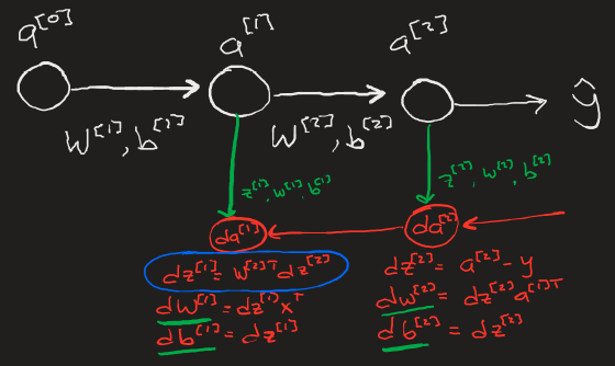
The key mechanism that makes deep learning powerful is Backpropagation which calculates the appropriate changes to all weights and biases in a neural network that will overall reduce the model’s cost function.

The simplest representation of backpropagation can be seen here, data from each neuron in each layer during the activation calculation stage is saved in a cache (Z, W, b) to then be used in the backpropagation calculations for the gradients dW, db.

In Practice

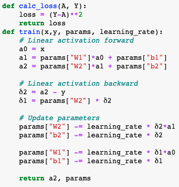
The code for a one hidden layer backpropagation is very simple. It consists of three distinct steps: forward propagation, backwards propagation, and parameter update.

1. Linear activation (forward) - [[MLBasics]] calculate the neuron’s activation vlaue with W * x + b for each layer.
2. Linear activation (backward) - calculate the change in the parameters for each neuron (δW = δL/δW, δb = δL/δb) that, when applied to said parameters will lower the models overall loss function.
3. Update parameters - reduce and save the input parameters to be used again in the next iteration.
   • W = W-δW*Ω
   • b = b-δ*Ω

Model Error

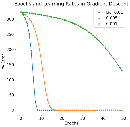
Passing the updated parameters back through the model is an “epoch”. As the epoch number increases, we’d expect the error in the model to diminish. We do in fact see this behavior as well as the same dependency on learning rate (lower learning rate makes for a slower learning neural network).

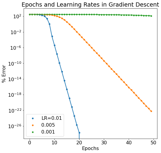
Below is a semilogy plot of the same data to reveal the discrepancy between the 0.01 and 0.005 learning rate models.

Next Steps

Next, we need to expand this backpropagation framework to allow for two things. First, we need to be able to add as many hidden layers as we want. Second, we need hidden layers to be modifiable to have any number of neurons. This will result in a fully modular deep learning neural network that can be easily modified on the fly.