Chapter 8 - Mathematical Modeling

8.3 Finite Difference Solution - Euler Method

The finite difference equation we need to solve is

More generally

Writing explicitly the finite difference expression in the LHS yields

Euler method results by solving the equation above for f(t+Dt), namely

For the radioactive problem, this translates into

The geometrical interpretation of this expression is that of an extrapolation of the unknown function from t to t+Dt via a straight line.

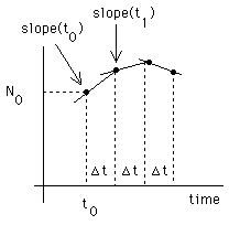
The idea is then to start from N(t) at the initial time, calculate the slope (rhs), then to calculate N(t+Dt) , and to repeat the steps as often as necessary to calculate the function over the desired interval. The steps to generate the unknown function are therefore:

1. specify the model ( equations ( rhs ) & constant ( k for the radioactive decay ) )
2. specify the initial conditions
3. define and set the time grid
4. repeat ( via a "for" loop ) the application of the Euler equation
5. store the results in arrays
6. visualize the solution via plotting

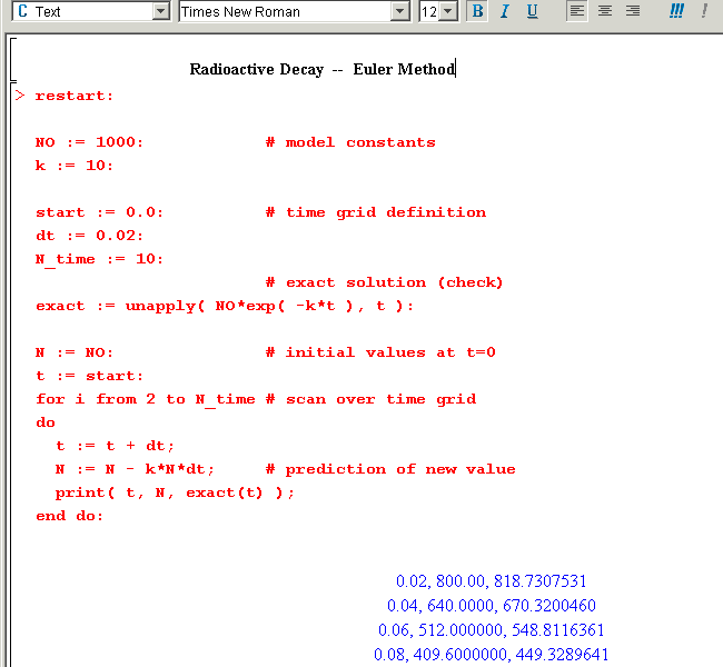
The following Maple worksheet implements the solution of the radioactive decay problem. The exact solution is also calculated for comparison.

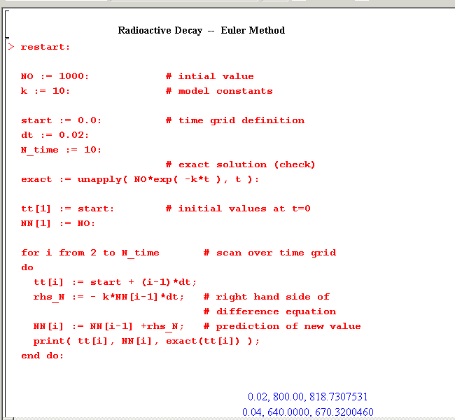
The following Maple worksheet stores the approximate solution in arrays and prints the approximate and the exact solutions. The solution follows the same logic as the one implemented in the simplest Maple worksheet above.

A better way to display the solution is via a plot:

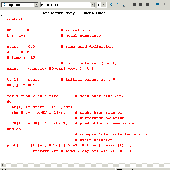
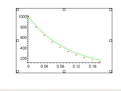
This last example can be downloaded from the web: Radioactive_Euler.mw

Any questions or suggestions should be directed to Michel Vallières at vallieres@physics.drexel.edu