

Once a function is calculated on a grid, a natural question to ask about the function is: What is the area under this curve representing the function? For instance, if the function represents the monthly revenue of a company, the area under the curve could be the annual revenue, if the area is calculated over a year period. If the function is a current, the area under the curve is a charge; if the function models a current flow, the area under the curve is the accumulated water in a reservoir. The "area under a curve" is clearly a very useful concept!
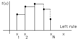
The question can be answered numerically via procedures based on simple graphical interpretations. For instance, the "left rule" corresponds to the following "cartoon", which translates in the formula given, and the Maple worksheet.

![]()
This formula can be easily incorporated in a Maple worksheet. (here, yy[k] contains the function values on the numerical grid, and there are N_points grid points - see the previous section for details)


![]()


![]()

These Maple blocks can be added to the Maple worksheet in the previous section which calculated the Skewed Mexican Hat function on a numerical grid to compute the "area under the curve". Here are the results.
![]()
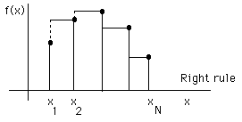
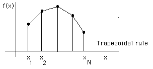
None of these numbers are exact, of course. The errors result from the fact that we approximated the underlying function by straight line segments. Look at the carton picture above and imagine those errors in the area as originating from the underestimation or overestimation of the area of the strips due to the area between the straight lines and the function.
In the next section, we will compare the results above to the exact one.
![]() Any questions or suggestions should be directed to
Any questions or suggestions should be directed to
Michel Vallières at vallieres@physics.drexel.edu