


Often times, one does not have an analytic expression for a function. For instance, suppose that a financial analyst has recorded the value of a stock on the stock market, twice a day for 30 days; this set of data does not likely correspond to some known function. Yet, the set of data defines a function, but numerically so. The rate of change of the stock value with time remains a valid question to ask. The limiting process explained in the previous section unfortunately does not apply in this case. In this section we will look for numerical procedures to implement approximate calculation of the slope. These will allow the calculation of the slope for functions given analytically or numerically.
A numerical description of a function is a tabulation of the function on a numerical grid. That is, the function is tabulated at regular or irregular values of x which cover the domain of the function. The following figure illustrates a function f(x) given on a regular numerical grid.
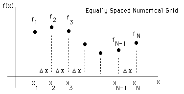
In the figure, f i = f( x i ) is the function at the ith grid point, x i = x min + (i-1) Dx.
Finite Difference Schemes
Finite Difference Schemes allow to calculate the slope of such a function which is tabulated on an equally spaced lattice. They make use of the tabulated function around the targeted x value. We will illustrate these formulae using Maple, and use arbitrary x interval, Dx, to illustrate the accuracy of such approximations. The function we will use to illustrate the method is the Skewed Mexican Hat, f(x) = x 4 - 3 x 2 - x.
The definition of the slope in Section 4.1 provides the Forward Difference formula.
The smallest Dx which can be used to compute the slope is often dictated by external circumstances, i.e., the interval at which data is measured. Therefore the limit implied by the mathematical definition of the slope can not be performed for a numerical function. Yet the form remain valid as an approximation.
The slope itself is a function of x, since the value of the value of the slope depends on the value of x at which the slope is calculated. Therefore it is natural to form a Maple function with the Forward Difference expression (done via the "unapply(,)" Maple command).
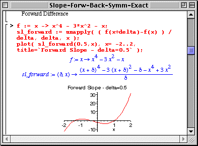
Note the regions of positive and negative slope in the figure; relate these regions to the shape of the Skewed Mexican Hat function.
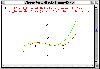
The Forward Difference slope function also depends parametrically on the interval used in calculating the slope; we expect a smaller Dx to yield a better value for the slope since it will be closer to the mathematical definition. Note that the "unapply()" command is used with two arguments, delta and x, to form a function of two variables. The following worksheet illustrates the d = Dx dependence of the slope function calculated with the Forward Difference formula.
The Backward Difference formula uses f(x) and f(x-Dx) to compute the slope.
The following illustrate this formula.
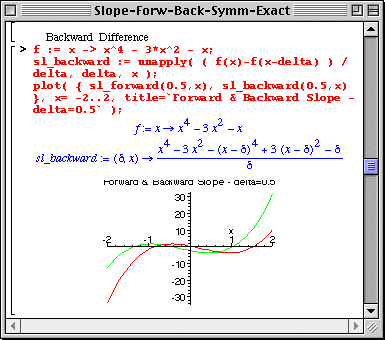
The Backward and Forward Difference formulae do not give the same values for the slope. Of course, if the mathematical limit Dx -> 0 could be taken, the two forms would be equivalent. Therefore, making Dx smaller should help bringing the two results closer; this is shown below.
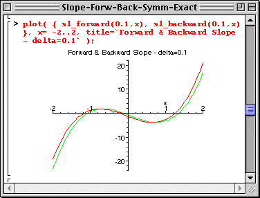
A much improved result can be calculated via using 3 lattice points instead of two, yielding the Symmetric Difference formula
That this is the case can be understood qualitatively from the following figure:
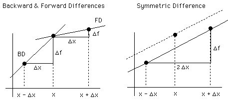
Imagine a "curve line" joining the points; clearly the Symmetric Difference form approximates the slope at x much better than the other two formulae.
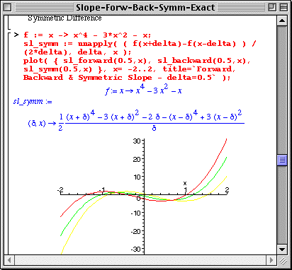
The Symmetric Difference formula gives a value for the slope function sandwiched between the Forward and Backward Difference formulae.
|
Any questions or suggestions should be directed to |