


In this section we present examples requiring the solution of non-linear equations. These will require slightly more complicated plotting capabilities from Maple.
The equations of a circle and of an ellipse are more easily written in implicit forms. An equation is said to be witten in implicit form when the x and y variables are mixed in the left hand side of the equation. For instance, the equation of a circle of radius R is
x2 + y2 = R2
This form is not easily plotted via the Maple plot( ) command. However, given the importance of these implicit forms, Maple provides for a special command to do this plot. It is called implicitplot(). The following illustrates its use for plotting a circle of radius R=1.
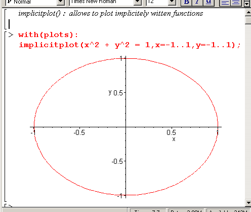
Note that the range is specified in both the x and y direction in this plot command. The circle does not apear rounded in this picture. To render the circle in a more natural way, you must force the axis to have same ratio; click on the plot, and select the 1:1 option.
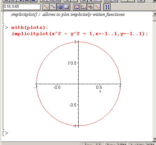
The command with(plots): loads the plotting library in Maple. The point is that some commands ( i.e., implicitplot() ) are not necessary for the average user of Maple. So why clobber the computer memory with more advanced and specialized commands when they are not used. The command with(library_name) loads these commands in Maple from the Maple libraries residing on disk. Note that issuing with(plots); will show you the list of commands loaded from the plotting library.
An ellipse is in some sense a deformed circle; the two axis i\of the ellipse have different lengths. The implicit equation for an ellipse is
x2 / a2 + y2 / b2 = 1
The following worksheet shows a circle of radius R=1 and an ellipse with a=2 and b=3. Note the { } brace notation which allows to plot the two curves simultaneously.
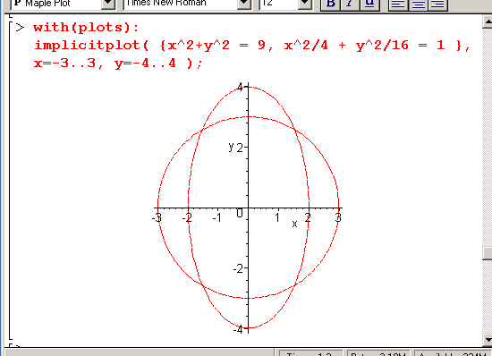
We now want to find the intersections of the circle and the ellipse in the figure above. An analytical solution for the intersection points does not exist. But a numerical solution is obviously possible. The fsolve(eqs,vars) is the command that allows to find these intersection points. You must "guide" fsolve() to the a right solution by specifying a range for the x and y variables. Here is how to do this:
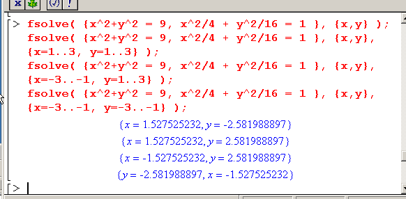
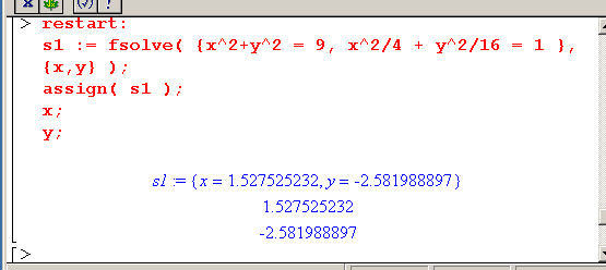
The solution of such an intricate system should be usable in further calculations within the Maple context. The first step to achieve this is to make Maple "remember" the values of x and y at the intersection points. The assign() command is what allows this. This command was illustrated in Section 3.1.
The fsolve() commands above echo statements which are list of equations. Therefore, assign() applied to the result of the fsolve() command will assign values to x and y. This is provided that the echoing of the fsolve() command is itself stored in some variables. The following Maple worksheet illustrates this:
A convenient illustration of the 4 interception points results from drawing a line joining these 4 points. The following is a Maple worksheet ( Circle-Ellipse ) that does precisely this. It also superposes the original circle and ellipse on the graph.
The unassign() command removes the assignment to a variable. A bit like restart, but for a single variable (or few variables) at a time. This is necessary in the worksheet due to the fact that the equations are writtern in terms of and solved for x and y. So, when solving for the second, third, ... intersection points the variables have no values.
The final plot is a combination of a graph done with the plot() command and one done with the implicitplot() command. The command display() allows the mixing of plot structures stored in different variables. Note that a necessary condition for this to be possible is that the x and y ranges be the same.
The reader should spend some time understanding in details this Maple worksheet. It is somewhat long, but the steps are relatively simple. The reader is also encouraged to read the Maple help panels on the assign(), unassign(), implicitplot(), and display() commands. Recall that typing ?command in Maple calls the help panel on any command.
|
Any questions or suggestions should be directed to |