


Solving one or more algebraic equations is often required in computational science. This is one of the basic operations in the field, and one of the easiest to understand intuitively. We all know what to do to solve a simple algebraic equation, i.e., 5*x+2=0; yet the equations encountered in real world models are rarely as simple as this and often present a challenge for the practitioner of computational science. Maple and Excel to the rescue!
Maple provides a very powerful equation solving environment. The basic syntax is:
solve ( eq, var );
where eq is an equation to be solved for the variable var. Systems of equations with many variables can also be solved using the syntax
solve ( eqs, vars );
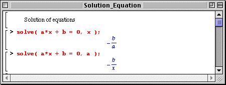
where eqs is a list of equations and vars is a list of variables to solve for. An equation is a "Left Hand Side = Right Hand Side" structure ( LHS = RHS ) where either or both LHS and RHS contains the unknown variables. The worksheet below illustrates the concept. Note that specifying the unknown to solve for is required, since who is to say which variable is unknown; it is only "customary" to label unknowns "x", "y", ... Maple remains general and does not assume this convention.
Maple also attempts to give the most general solution in every case. For instance, no assumption is made on the values of "a" and "b" in the worksheet below; depending on specific values of "a" or "b", either real (b/a negative) or imaginary (b/a positive) solutions are obtained. Maple denotes sqrt(-1) by I. Also note that two solutions exist for this equation, both found by Maple.
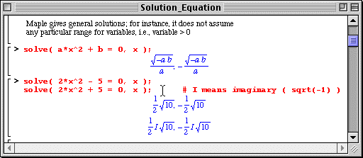
Maple is quite able to solve more complicated equations; do you recognize the following example?

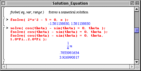
Maple can also solve equations numerically; the command is "fsolve()". The syntax is very similar to that of the solve command:
fsolve ( eq, var , range);
or
fsolve ( eqs, vars , range);
The range, min..max, is optional. Specifying a range often renders the numerical search for a solution more efficient for Maple, thereby using less computing (CPU) time. It may also be necessary to specify a range to find particular solutions in specific ranges of the independent variable in cases when multi-solutions exist.
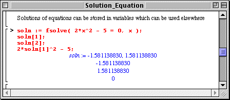
The solutions of equations can be assigned to variables and used in any other Maple command. Maple uses an "array" notation to store the solutions in cases when there exist multi-solutions. The different solutions are stored under a single name; each one is individually accessible via the notation
name[index]
where "index" numerically points to a particular solution; for instance, name[1] and name[2] would be the first and second solution of a multi solution case.
Maple can solve multi-equations systems of algebraic equations for many unknowns.
Both "solve()" and "fsolve()" can handle system of equations. The "sets" of equations are entered directly in the commands or first assigned to variables. In the worksheet below, the equations and variables are first entered in the "solve()" and "fsolve()" commands directly via the "{}" notation.

In the last example, eq1 and eq2 are assigned one equation each of a pair of equations, while eqs is assigned the 2 equations in a "sets" notation. The same for vars which is assigned the "sets" {x,y} of unknowns.
If the equations are linear, first power in the unknowns, a single solution (single value for each variable) may exist. In general, for nonlinear equations, multi-solutions may also exist.
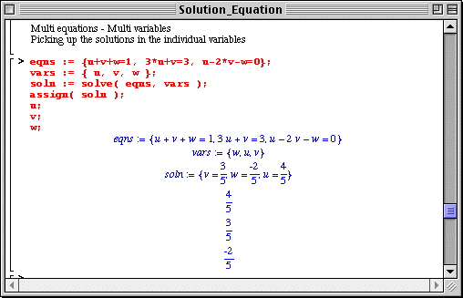
The solutions of a set of equations are themselves sets of values for the various unknowns. Maple allows to assign the value to each variable directly from the solution of the set of equations. This is done by the "assign" command. This command uses an equation type syntax to assign the RHS of the equation to the LHS of the equation; the latter must, of course, contain a single variable name. In the case of the solution of a set of equations, Maple understand the "sets" notation, i.e., { x=a, y=b }, and implements the multi-assignments at once. This is illustrated below.
|
Any questions or suggestions should be directed to |