

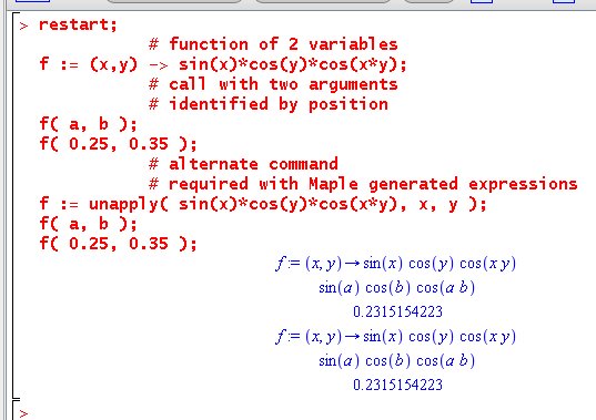
Functions of two independent variables are easily defined in Maple. Either the -> or the unapply(,) commands generalize trivially for this purpose:
name := ( var1,var2) -> expression;
name := unapply( expression, var1, var2 );
In either cases, name is the name of the function, var1 and var2 are the independent variables and expression defines the map. The function is used via
name( var_a, var_b )
The association var_a <=> var1 and var_b <=> var_2 is though the positions of the variables in the definition and call.
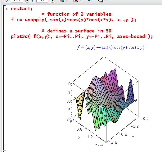
A function of two independent variables, f(x,y), defines a surface. Given numerical values for x and y, the function f(x,y) maps these values of x and y into a number. This can be done on an x-y grid from which Maple can draw the surface. The command
plot3d( f(x,y), x=range_x, y=range_y, options )
plots the surface specifiied by f(x,y) in the x-y domain specified by range_x and range_y using a default 25x25 grid.
Note that Maple allows full control over the graph and the observation point. A mouse click on the graph enables options to appear in the top bar. You should explore the variaty of textures and axes that are available. You should also "grab" the surface and rotate it. This provides an amazing tool to study any surface by allowing you to inspect the surface from any angle.
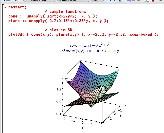
The command is also capable to display multiple surfaces at once. The following worksheet shows how easy it is to display a cone intercepted by a plane. Note how simple the syntax is and how it contitutes a simple generalization of what we saw for the plot() command.
The command also accepts many options. For example, the option grid=[m,n] where m and n are positive integers, specifies that the plot is to be constructed on an m by n grid at equally spaced points in the x and y ranges respectively. By default, a 25 by 25 grid is used and 625 points are generated. Other options include specification of alternate coordinate systems and rendering styles. For more information, see ?plot3d,options.
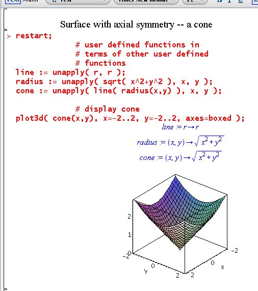
Maple allows full analytical manipulations with functions of multi variables. For instance the following worksheet illustrates how the axial symmetry property of a cone can be used in its definition. Functions of one and two variables are used as arguments of each other.
Maple allows the definition and use of multi-variables functions. This is exemplified in the next worksheet with a function of three variables.
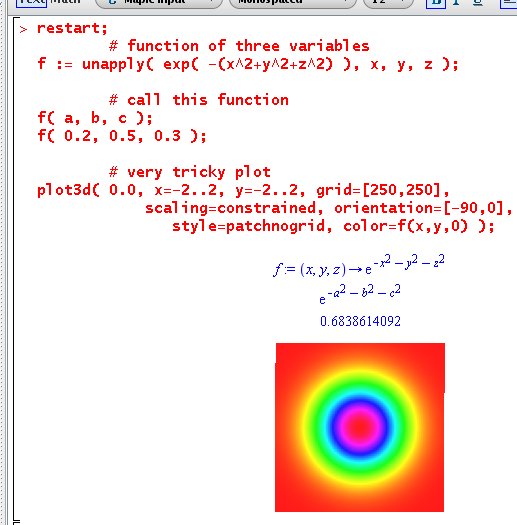
The plotting of such functions can be tricky or impossible (we live in 3D). One way to "see" functions of multi-variables is via slices through the data. For instance f(x,y,0) selects a slice of the function in the plane z=0. The command plot3d(,,) can be used in "contour" mode, in a specific x-y domain, with the color display being defined by the function f(x,y,0) itself. To see the contour plot, the constant function 0.0 is plotted and looked at from an observation point above the plane, orientation=[-90,0]. The color and contour values are therefore plotted in this plane (z=0.0) with no distorsion. The x-y grid is refined by specifying grid=[250,250] instead of the default 25x25 size. Reading the help ?plot3d,options will help understanding this complicated plot!
|
Any questions or suggestions should be directed to |