
In this section we present various more complicated examples requiring the solution of equations; the reader is encouraged to think about these problems, define the equations in Maple, and attempt a solution before downloading the complete solutions for comparison. These solutions do not require more advanced concepts or Maple/Excel syntactic rules than presented earlier in the chapter.
A financial analyst has analyzed the performance of a stock on the Stock Market; he has fitted the stock value over a period of 20 months using the following form
The constants are
|
a_k |
a_k |
b_k |
|
|
k = 1 |
10.5 |
5.5 |
7.3 |
|
k = 2 |
6.5 |
11.1 |
1.9 |
|
k = 3 |
9.5 |
15.5 |
28.5 |
Find the time intervals during which the stock value was over $9.00. Those were the "good times"!
Solution: Stock_Price.
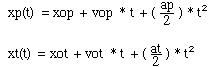
A robber drives past a police car which is cruising at low speed (20.1 m/sec) in some neighborhood. By the time the police officer reacts to start the pursuit, the thief is already 50 m away and going at 85.6 m/sec; at that moment we start measuring the time. The police car is powerful and can accelerate much better than the thief's car and so the police officer sets out to catch the robber. The equations describing the positions of the police car, xp(t),and the thief's car, xt(t), as a function of the time t are:
The constant quantities (initial conditions) have values:
|
Police Car |
Thief's car |
|||
|
initial position (m) |
xop |
0.0 |
xot |
50.0 |
|
initial velocity (m/sec) |
vop |
20.1 |
vot |
85.6 |
|
acceleration (m/sec/sec) |
ap |
40.3 |
at |
7.5 |
Question: At what time and where will the police catch up to the thief?
Solution: cop_catching_up_thief.
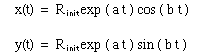
When NASA wants to have the space shuttle reenter the atmosphere, it simply slows it down slightly below the orbital speed, after which the space shuttle spirals down to earth. We will model this reentry orbit.
We will neglect the air resistance slowing down the shuttle, and we will assume that the shuttle moves in a plane passing through the earth's equator to simplify (considerably) the solution. The parametric equations for the spiral are:
Assume: R_earth = 1.0, R_init = 2.0, a = -0.3, b = 5.0, and t_init = 0.0 (all scaled units, i.e., distances in earth radius unit).
Where and when does the Space Shuttle land?
Hints: Define the shuttle position coordinates, x(t) and y(t), as functions in Maple - plot the position of the shuttle around the earth (draw a circle representing the earth) - find the height (distance from the earth center) of the shuttle as a function of time - plot the height of the shuttle as a function of time - solve for the landing time - find the landing position.
Solution: Shuttle_Spiral_Orbit.
|
Any questions or suggestions should be directed to |