

The best intuition about mathematical functions is gained by plotting. Maple provides very powerful tools to accomplish this task, for simple x-y all the way to quite sophisticated 3-D plots.
The syntax for plotting is quite simple and intuitive. For instance, an x-y plot is obtained via the basic syntax
plot( function, range );
or
plot( {function_1, function_2 }, range );
or
plot( [function_1, function_2 ], range );
The range is specified by the syntax:
variable = min..max
The plot defaults to a range {-10,10} if no range is specified. The {,} or [,] notation is used to plot more than one function. The {,} generates a set out of its arguments while the [,] generates a list. See ?set for help and examples.
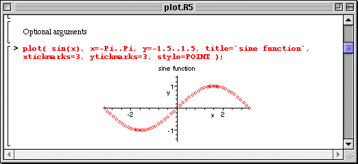
Here are some x-y plot examples using trigonometric functions (the # is followed by comments - these are useful for later understanding one's work, or for clarifying one's work for others).

Note that the default for Maple is to plot within the worksheet. This is very convenient in order to print the results of a calculation. However, Maple can also plot in separate windows by selecting this option from the "Options" menu, choosing from within "plot display" sub-menu. This is the best option to use while developing a new worksheet. Once satisfied with the results, one can run the calculation again to include the graphs in the worksheet.
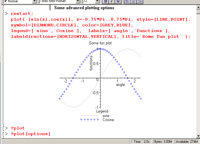
The plot command also accepts more specialized arguments, which are well explained in the help panel for the "plot" command (?plot and ?plot,options). Most of these options can be intuitively understood. Some of these are illustrated below.

The [,] notation for the functions extends to the list of parameters. The list members correspond to the list of functions and should be quoted in the same order. The exception is in specifying values for the labels and labeldirections ketwords; in this case the two entries correspond to the x- and y-axis values. Note that the string of characters in the labels entries are surrounded by back quote charaters to allow special characters, i.e., spaces, to be used. The following worksheet illustrates this.

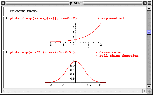
An interesting function which we will need later is the exponential function, the inverse of the natural logarithm. It is called via
exp(arg).
Here is how it looks:

The Gaussian function or Bell Shape function is important in many fields; it often appears in statistic applications. It is a simple exponential with a quadratic argument. It produces a very characteristic bell shape.
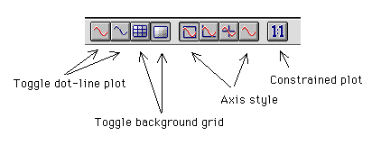
A "graph" menu appears to allow plotting style selection once a graph is made active by clicking on it (by bringing the separate window in the foreground). These buttons have obvious meanings for the most part. The "constrained plot" option toggles between a plot drawn to optimize the use of the Maple window and one in which the ratio data/graph distance is the same in both directions in the window. For example, this option allows to draw a "real" circle on the screen.

Maple excels at plotting more complicated functions, even in 3-D. Here are two fine examples; try them yourself and see how Maple allows you to rotate the shapes quite arbitrarily. We will likely not need such sophisticated Maple capabilities in this text, yet it is good to know that advanced plotting facilities exist in Maple and that they are easy to use.
|
Any questions or suggestions should be directed to |