
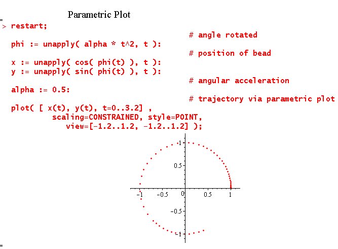
The trajectory of the point on the rim of a wheel that is speeding up is illustrated below via the Maple parametric plot command. The x- and y-coordinates of the point are given by the x(t) and y(t) functions that depend (parametrically) on time. The trajectory is generated by plotting y(t) versus x(t). The syntax can be deduced from the help panel generated by ?plot[parametric].
In this example, the command generates values of the parameter t in the range t=0..3.2. The positions of the point (values of x(t) and y(t)) are automatically generated and displayed through the graph. The scaling=CONSTRAINED option in the plot command is to invoke the 1:1 scaling - to make the trajectory appear as a circle, which it is. The view option sets a viewing window.
The point on the rim starts from rest on the positive side of x-axis. As time passes, the point rotates counter-clockwise. The dots on the figure become further apart (same time interval between the dots) since the speed of rotation of the wheel increases (linearly) with time.
Maple is an exceptionaly versatile package for plotting functions. It is equally capable to produce animations.
The command animate in the plots library allows to animate a variety of plot commands. The syntax is
animate( plot_command, [arguments], parameter=range );
This animates the command plot_command(arguments) over the specified range of the parameter. The arguments of the plot() command are placed in [] in 2nd position in the animate command.
For instance, the worksheet below animates a gaussian curve over a range of width. The statement
plot( gaussian(x), x=-3..3 );
would plot the gaussian function of standard width. gaussian(alpha*x) are gaussian functions of width controled by the parameter alpha. Therefore, the animate() statement makes a "movie" based on gaussians of different width in each frame.

Try this for yourself - download Gaussian_movie.mw. Note that clicking of the graph awakes the movie control buttons, e.g., stop, play, ..., in the top bar.
The trajectory of the point on the rim of a wheel that is speeding up is illustrated below via an animation created by Maple. The idea is to animate the trajectory based on an increasing time of the last point on the trajectory.
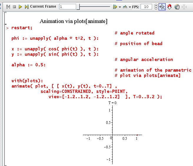
Try this for yourself - download traj_animate.mw.
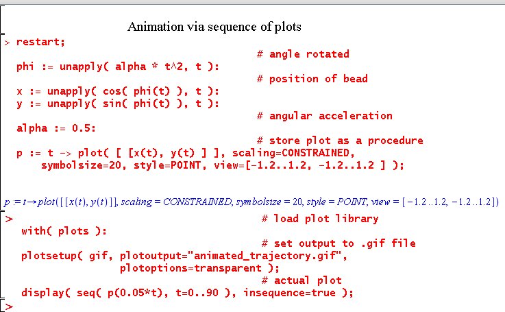
The animation above is easy, but not really the best. It would be more natural to see the point on the rim of a wheel itself move along the trajectory. This is illustrated below via an animation created by Maple. This application is much more intricate than a novice is normally expected to know. Yet it is reassuring and satisfying to realize that Maple is a very capable package, able to render very sophisticated graphics.
The basic idea is to create a function of t which is a plot of a single point corresponding to the position of the point on the rim at time t. Then a series of plots is generated via seq(exp,range). These are displayed via the display() command, in which the parameter insequence is set to TRUE so as to display the plots in sequence.
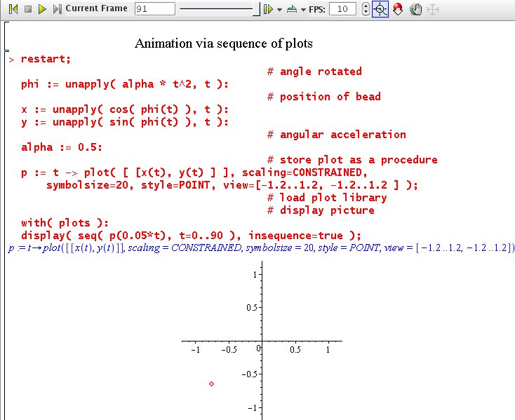
Note that seq() generates a sequence of integers, which are transformed in a reasonable time range by multiplying by a factor 0.05.
You can try them yourselves by downloading the Maple worksheet to your computer ( traj_seq_plots.mw ).
The animated graphic can be transferred into an animated GIF file via specifying the output device to be a GIF file for the display command. The command plotsetup() is used for this purpose.
The result is a GIF file which can be viewed via a browser.
The commands used here are quite complicated; they accept many more options than those shown. This section is meant to be complemented by the Help files from Maple for the serious reader who needs to use these more sophisticated graphic capabilities.
|
Any questions or suggestions should be directed to |