6.  Varying the time step in N-body applications

1. Knowing the physics

   • We can define several time scales for an N-body system:
     Note that these quantities all have dimension of time, and they represent estimates of how rapidly particles i and j can cross the distance between them. The first two represent simple crossing times (distance divided by relative velocity), the third the free-fall time (square root of distance divided by acceleration). If we have access to these quantites during the integration (which we do in our N-body code, but generally don't in a canned integration routine), then we can compute a characteristic time scale for the entire system at the same time as we compute the accelerations (the "ij" quantities are only known inside the force calculation loop).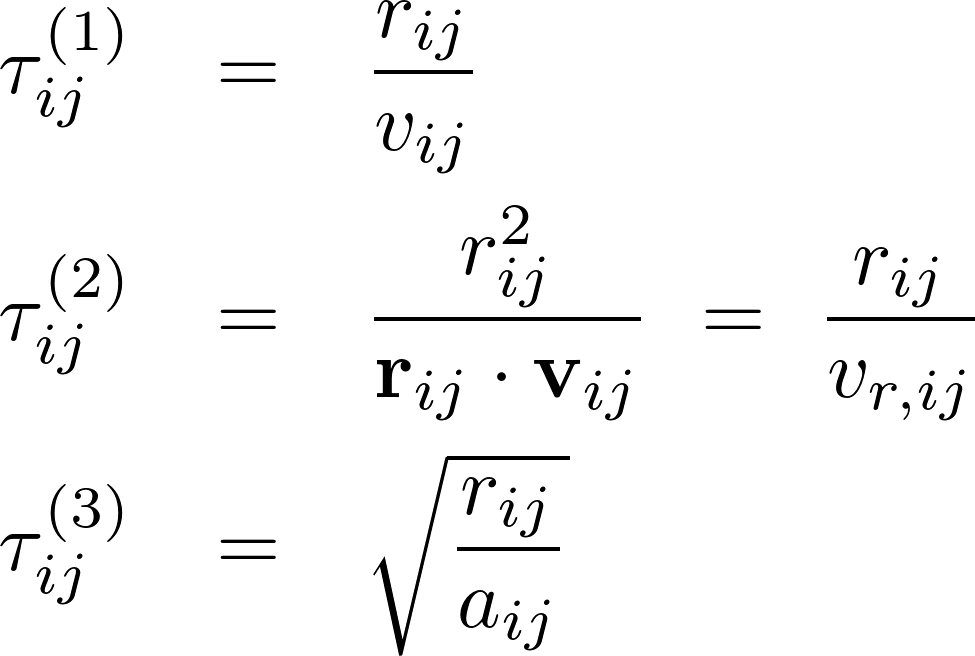

     The basic approach is then to take some fixed multiple of this time scale (0.01, say) as our time step, making our integrator adaptive. This works because, if we consider just the radial acceleration, we find

     so the "jerk" error term 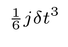is just the cube of the time step divided by a combination of the time scales defined above.

   • Exercise 6.1:  Let's start with something simpler, and just look at the 2-body problem and only the third time scale. Since there is only one pair (0, 1) and
     we find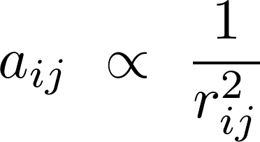
     or scaling to some convenient time step at some separation: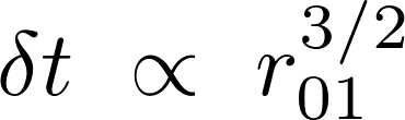
     Repeat exercise 5.1, but this time adjust the time step after every step using the above formula. Take dt0 = 0.01, v0 = 0.09, eps = 0, and run to time t = 50. Note that the variable time step scheme is (a) much more accurate than the fixed time step scheme, and (b) no longer time reversible. Which of these is more important depends on the application. Gravitational N-body people can generally live with the non-reversibility, while molecular dynamicists and planetary scientists usually insist on a reversible integrator.   (Solution.)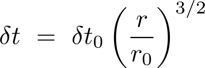

     • Find an accuracy parameter in Exercise 6.1 that leads to a maximum error during the run of less than 0.0001.   (Answer: 0.0085.)

     • Find a fixed time step in Exercise 6.1 that leads to a similar maximum error during the run.   (Answer: 0.00025.)

   • Exercise 6.2: Modify the acceleration routine in your code to compute and return the instantaneous time scale tau defined by
     That is, every time the accelerations of particles i and j are calcluated, also compute the two time scales and determine the minimum time scale across all pairs. This will require the value of tau to be propagated through two functions. A slightly modified version of the previous solution, which propagates tau through the step and acceleration functions but doesn't actually compute it, is provided here. Complete the code to compute tau and plot its value as a function of time along the orbit. Don't use tau yet to vary the time step. That will be the topic of the next exercise.   (Solution.)

   • Exercise 6.3: Now implement the full variable time step scheme, using tau as just defined, and apply it to the same 2-body system as in the previous two exercises. That is, multiply tau by a time step parameter eta (set by default and/or on the command line), which can be adjusted to fine-tune the energy error.   (Solution.)

   • Exercise 6.4: Now use the scheme just created to solve a small N-body problem. Create a system of N = 20 identical particles with total mass 1, initially distributed in a homogeneous sphere of radius 1, with initial speeds v = 0.1 distributed isotropically in direction. Choose an initial numpy random seed of 12345 and be sure to initialize the system in the center of mass frame. Use a softening parameter eps = 0.01 and run the calculation until t = 5 time units. Print out the time and energy error |E - E0| (where E0 is the initial total energy) at intervals of 0.25 time unit, and find a value of eta that ensures an energy error (checked every 0.25 time units) of less than 1.e-4 throughout the run. How many total time steps does the calculation take?

     Here are some notes on using numpy to generate random points and velocities.

2. Time step doubling

   • read Numerical Recipes in C, Sec. 17.2

   • A less intrusive and more "algorithmic" way to control step sizes is a technique known as step doubling. In this approach we need know nothing about the details of the calculation, only the order of the integration scheme. For example, we know that the predictor-corrector scheme we have been using is second order, meaning that the error at the end of a step is of order phi dt^3, where phi is roughly constant over the step (one sixth the jerk, in this case). After every two "normal" steps of length dt, we repeat the calculation by taking a third step of length 2dt spanning the same interval. If we denote the true solution by y and the numerical solutions with one and two steps by y1 and y2, we can say

     	    y = y1 + phi (2dt)^3 y = y2 + 2 phi dt^3

     assuming that the errors in the two shorter steps simply add. Thus we find

     	    Delta = y2 - y1 = 6 phi dt^3

     that is, we can measure phi directly from the numerical data.

     The trick then is to adjust the time step to keep the error constant. This sounds straightforward, but it reveals the downside of keeping our fingers out of the code -- we have to decide (or in a canned implementation, somehow tell the integrator) exactly what the error is that we want to limit. In this case, we could elect to limit the error in the position, or the velocity, or both, or some combination of the two. The choice is not always obvious. Here, we have been focusing on energy conservation, so it makes sense to scale the step to keep the energy error per step constant.

     In other words, after we take the short and long steps, we calculate the energy after each:

                 t0 = t
                 pos0 = pos.copy()
                 vel0 = vel.copy()
     
                 t,pos,vel = step(t, mass, pos, vel, eps**2, dt)
                 t,pos,vel = step(t, mass, pos, vel, eps**2, dt)
                 E1 = energy(mass, pos, vel, eps**2)
             
                 t2,pos2,vel2 = step(t0, mass, pos0, vel0, eps**2, dt2)
                 E2 = energy(mass, pos2, vel2, eps**2)

     We then define

     	    DeltaE = abs(E2 - E1)

     and we scale dt to keep DeltaE fixed at some value dEtol, i.e. we choose the next step according to

     	    dtnext = dt*(DeltaE/dEtol)**(-1./3)

     This should properly scale the step to force the error back to the desired value. You'll need to experiment with dEtol until the desired global accuracy is obtained. Note that the order of the method enters directly into the scaling through the -1/3 exponent.

     One conservative caveat: you could in principle just accept dtnext as the new step, but it is usually advisable to limit changes in dt, just in case something unexpected happens. I prefer to accept dtnext if it is less than dt (it's always OK to take too short a step), but to limit the growth of dt as a precaution. The logic is:

                 if dtnext > 1.5*dt:
     		dt = 1.5*dt
     	    else:
     		dt = dtnext

   • Exercise 6.5: Implement a step-doubling scheme for the same two-body system as studied in the previous three exercises. Adjust dEtol until the overall error is roughly the same as before -- 0.0001 -- and compare the total number of steps taken in each calculation. (Don't count the double-length step as an extra step.)

   
   Homework #4

   
   

3. Embedded schemes

   • Numerical Recipes describes an alternative way to estimate Delta using a so-called embedded scheme -- a Runge-Kutta integrator in which the data can be combined in two different ways to obtain (say) fourth- and fifth-order schemes with no additional work. Since the schemes have different order, comparing y4 (the numerical result from the fourth-order scheme) and y5 (the fifth-order result) again allows an estimate to be made of the error. Once that estimate is in hand, we proceed to adjust the time step in much the same way as for step-doubling.

   • read Numerical Recipes in C, Sec. 17.2

   • Here's a sample Butcher tableau: