RLC Circuits

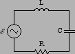
Electrical circuits are more good examples of oscillatory behavior. The general circuit we want to consider looks like

which, going counter-clockwise around the circuit gives the loop equation

$$\mathscr{E}-IR-\frac{q}{C}-L\frac{dI}{dt}=0,$$

where $I$ is the current in the circuit, and $q$ the charge on the capacitor as a function of time.

We note that $I=dq/dt$ and $dI/dt=d^2q/dt^2$, so that our equation becomes

$$L\frac{d^2q}{dt^2}+R\frac{dq}{dt}+\frac{1}{C}q=\mathscr{E}(t),$$

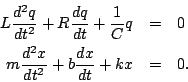
and we will first look the undriven case $\mathscr{E}=0$. This gives the following equation

$$L\frac{d^2q}{dt^2}+R\frac{dq}{dt}+\frac{1}{C}q=0,$$

which should be familiar - a second degree ordinary differential equation with constant coefficients. We saw this same equation when we studied damped motion. In fact, this is the same equation and describes essentially the same phenomenon. Let us compare:

$$\begin{eqnarray*} L\frac{d^2q}{dt^2}+R\frac{dq}{dt}+\frac{1}{C}q &=&0\\ m\frac{d^2x}{dt^2}+b\frac{dx}{dt}+kx &=&0. \end{eqnarray*}$$

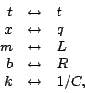
It doesn't take long to see that the equations are identical with the following correspondence:

$$\begin{array}{rcl} t &\leftrightarrow & t \\ x &\leftrightar... ... &\leftrightarrow & R \\ k &\leftrightarrow & 1/C, \end{array}$$

where we simply compare term-by-term. NOTE that it is the capacitor that corresponds to the spring not the inductor, even though the picture of an inductor looks like a spring!

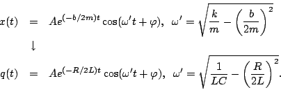
So, charge is like displacement, inductance like mass (inertia), resistance like damping, and capacitance like compliance (inverse springiness). Now that we have the variable correspondence we can write down the solution by comparison:

$$\begin{eqnarray*} x(t) &=& Ae^{(-b/2m)t}\cos(\omega't+\varphi),\;\;\omega'=\sqrt... ...hi),\;\;\omega'=\sqrt{\frac{1}{LC}-\left(\frac{R}{2L}\right)^2}. \end{eqnarray*}$$

So the behavior of our circuit is characterized by damped oscillations of the charge on the capacitor.

Note that when we have no resistance ($R=0$), our equation simplifies to

$$\frac{d^2q}{dt^2}=-\frac{1}{LC}q,$$

which is the equation for simple harmonic motion with frequency

$$\omega^2=1/LC.$$

Now, it is in general very difficult to solve this equation when $\mathscr{E}\neq 0$. An important method is the Laplace Transform, which turns our differential equation into an algebraic one, which is (hopefully) easier to solve. Conceptually you get the following:

where $\mathscr{L}$ stands for the Laplace transform and $\mathscr{L}^{-1}$ its inverse. In any case, if we take a sinusoidal emf $\mathscr{E}=\mathscr{E}_0\sin(\omega_dt)$, then the above procedure tells us that we obtain a state of resonance in the circuit when

$$\omega_d^2=\omega_0^2-2\left(\frac{R}{2L}\right)^2,$$

where $\omega_0^2=1/LC$, which is just a little bit different from what we'd expect. The stuff on the right is the 'natural frequency' of the circuit, but we're going to assume that $R$ is small enough that the resonance frequency is simply given by $\omega_0$. How small? Well, we need that second frequency in the above equation to be very small compared to the first, or

$$\frac{R^2}{2L^2}<<\frac{1}{LC},$$

which, when solved for $R$ gives

$$R<<\sqrt{\frac{2L}{C}}\approx \sqrt{\frac{L}{C}},$$

since $\sqrt{2}\approx 1$ (order of magnitude). We will even assume $R$ to be 'small' so that we can solve for it nicely in one problem. It's a good idea to go back, after finding $R$, to make sure it actually does satisfy this condition, otherwise the assumption was wrong and our value of $R$ is no good!